Michele Coscia

When you’re studying complex systems, one of the most important questions you might have is: how will this system evolve in the future? If you’re modeling your system as a network — as I like to do in my spare time — this boils down to predicting the arrival of new nodes and links. This is the realm of link prediction. In this post, I’ll describe one advancement in the field that I developed with fellow NERD Michael Szell in the paper “Multiplex Graph Association Rules for Link Prediction“, to appear next year at the ICWSM conference.

There are many ways to predict new links in a network, but most of these methods have a disadvantage: they can only give you a score for potential future connections between two nodes that are already in the network when you observe it. In other words, they cannot predict new incoming nodes. But with a technique called “graph association rules”, used by the GERM algorithm published in 2009, we can predict new nodes. How is that possible?

In simple terms, a “graph association rule” is a rule that tells you: every time you see in your network a pattern A, it will turn into pattern B, with a certain degree of confidence. The rule is extracted by counting how many times patterns A and B appear. For instance, in the image below, if pattern A (the triangle) appears 9 times and pattern B (the triangle with a dangling node) appears 6 times, the confidence of the rule is 2/3. 66% of the time, a triangle has attracted a dangling node. Note that pattern B must include pattern A, otherwise it’s difficult to hypothesize that A evolved into B.

GERM has a problem of its own, which Michael and I set out to solve: it can predict incoming nodes and links, but it cannot distinguish between different link types. In other words, every predicted link is the same to GERM. However, many real world networks have link types: nodes can connect in different ways. For instance, on social media, you connect to the people you know in different ways: via Facebook, Twitter, Linkedin, etc.

You’d model such system with a multiplex network, which allows for link types. If you have a multiplex network, you need multiplex graph association rules for link prediction. Which is exactly the title of our paper! What a crazy coincidence!

In the paper we re-purpose Moss, a graph pattern miner that can extract multiplex patterns, to build such rules. We created a pre- and post-processor of Moss that can construct the rules based on the patterns it finds. Now we can give colors to the links that are featured in our rules, as the figure below shows. This is a generalization of the signed link predictor I already wrote about a long time ago (the second ever post on this blog. I feel old).

Doing so isn’t painless though. We made sacrifices. For instance, our rule extractor doesn’t really understand the passage of time. It knows that the input network is in the past and spits out the rules to predict its evolution, but it doesn’t know how long a rule will take to complete. Unlike GERM, which can tell you that a rule will take n timesteps to complete.

This downside is minor though. Our link predictor performs well, as witnessed by the ROC curves below (our method in red). The comparisons are other multiplex link predictors. Not only are they worse at predicting links, but they have the added disadvantage of being unable to predict the arrival of new nodes. They also have issues with memory consumption, because they generate a score for each pair of nodes that is not connected in the training data — which, for sparse networks, is a lot of scores. Our predictor, instead, only gives scores to the links that are valid consequences of the rules that we found, usually way fewer than all unconnected node pairs.

If you want to play with our link predictor, you can do so by downloading the code I made public for the replication of the paper’s results. The code is very academic — meaning: badly written, unreasonably fragile, and horribly inefficient. I have in the works an extension with more efficient and robust code, and a generalization from multiplex to fully multilayer networks. Stay tuned!

Continue Reading

If there is a thing that I love more than looking at silly pictures on the Interwebz for work is to watch rugby for work. I love rugby: in my opinion it is the most beautiful team sport out there. It tingles my network senses: 15 men on the field have to coordinate like a single organism to achieve their goal — crossing the goal line with the ball by passing it backwards instead of forward. When Optasports made available some data collected during 18 rugby matches I felt I could not miss the opportunity for some hardcore network nerding on them. The way teams weave their collaboration networks during a match must have some relationship with their performance, and I was going to find out what this relationship might be.

For my quest I teamed up with Luca Pappalardo and Paolo Cintia, two friends of mine who are making an impact on network and big data sports analytics, both in soccer and in cycling. The result was “The Haka Network: Evaluating Rugby Team Performance with Dynamic Graph Analysis“, a paper recently presented at the DyNo workshop in San Francisco. Our questions were:

1. Is there a relationship between the topology of the network of passes and the success of the team?
2. Is there a relationship between disruptions made by tackles and territorial gains?
3. If we want to predict a team’s success, is it better to build networks of passes and disruptions for each action separately or for the entire match?
4. Can we use these relationships to “predict” the outcome of the match?

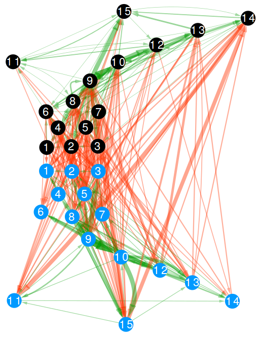
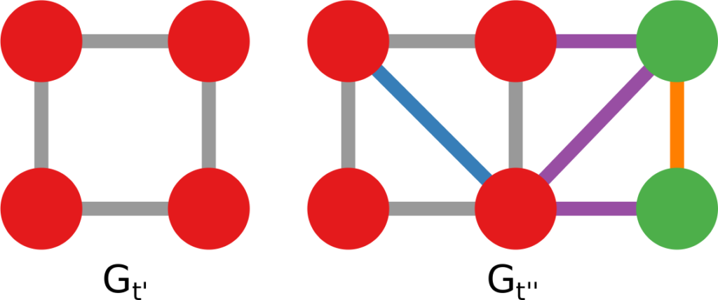
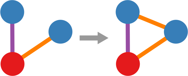
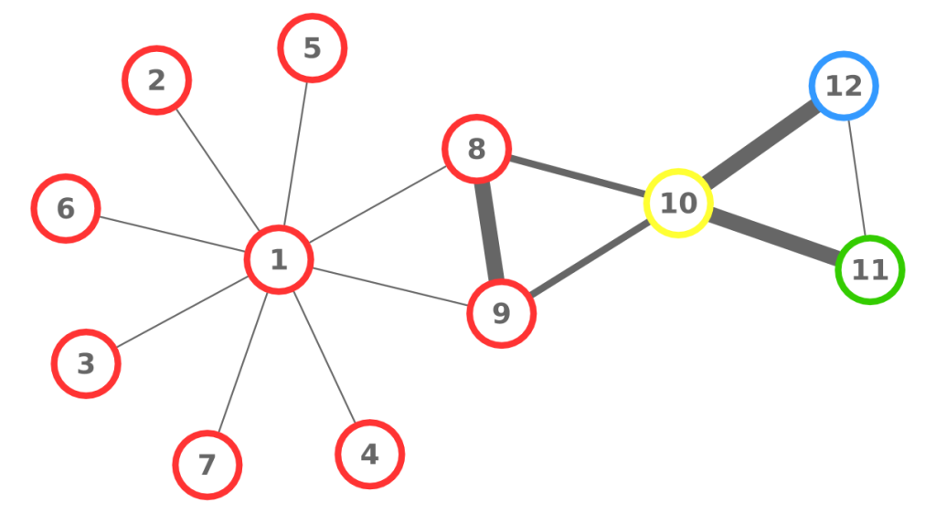
A passage network is simply a network whose nodes are the players of a team and the directed connections go from the player originating a pass to the player receiving the ball. We consider only completed passages: the ones that did not result in an error or lost possession. In the above picture, those are the green edges and they are always established between players belonging to the same team. In rugby, players are allowed to tackle the current ball carrier of the opponent team. When that happens, we create another directed edge, this time in what we call “disruption network”. The aim of a tackle is to prevent the opponent team from gaining meters. These are the red edges in the above picture and can only be established between players belonging to opposite teams. The picture you see is the collection of all passes and tackles which happened in the Italy vs New Zealand match in 2012. It is a multilayer network as it contains edges of two different types: passes and tackles.

Once we have pass and disruption networks we can calculate a collection of network measures. I’ll give a brief idea here, but if you are looking for more formal definitions you’ll have to search for them in the paper:

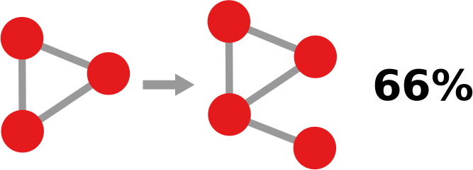
• Connectivity: how many pass connections you have to remove to isolate players;
• Assortativity: the tendency of players to pass the ball to players with a similar number of connections — in high assortativity central players pass to other central players and marginal players to other marginal players;
• Components: how many “sinks” there are, in that the ball never goes back to the bulk of the team when it is passed to a player in a sink;
• Clustering: how many triangles there are, meaning that the team can be decomposed in many different smaller sub-teams of three players.

These are the features we calculated for the pass networks. The disruption case is slightly different. We calculated the same features for the team when removing the tackled player, weighted on the relative number of tackles. If 50% of the tackles hit player number 11, then 50% of the disrupted connectivity is the connectivity value of the pass network when removing player 11. The reason is that the tackled player is temporarily removed from the game, so we need to know how the team performs without him, weighted on the number of times this occurrence happens.

So, it is time to give some answers. Shall we?

1. Is there a relationship between the topology of the network of passes and the success of the team?

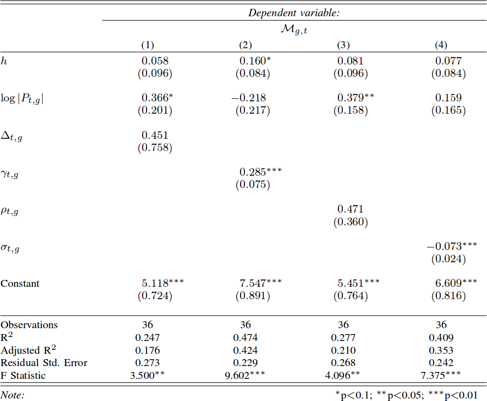
Yes, there is. We calculate “success” as the number of meters gained, ball in hand, by the team. The objective of rugby is to cross the goal line carrying the ball, so meters made is a pretty good indicator. We control for two things. First, the total number of passes: it simply means the team was able to hold onto the ball longer, so it is trivially expected to result in more meters. Second, the home advantage, which is a huge factor in rugby: Italy won only 12 out of 85 matches in the European “Six Nations” tournament, and 11 of them were in Italy. After these controls, we find that two features have good correlations with meters made: connectivity and components. The more edges are needed to isolate a player, the more meters a team is expected to make (p < .01, R2 = 47%). More sinks in a team is associated with lower gains in meters.

2. Is there a relationship between disruptions made by tackles and territorial gains?

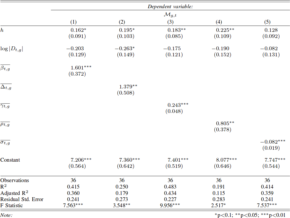
Again: yes. In this case it seems that all calculated features matter to predict meters made. The strongest factor is again leftover connectivity. It means that if the connectivity of the pass network increases after the tackled player is removed from it then the team is able to advance more. Simplifying: if you are able to tackle only low connectivity players, then your opponent is able to gain more territory (p < .01, R2 = 48%).

3. Is it better to build networks of passes and disruptions for each action separately or for the entire match?

The answer to the previous two questions were made by calculating the features on the global match networks. The global network uses all the data from a match, exactly like the pass and disruption edges depicted in the above figure. In principle, one could calculate these features as the match unfolds: sequence by sequence. In fact, networks features at the action level work very well in soccer, as Luca and Paolo already proved. Does that work also in rugby?

Surprisingly, the answer is no. We recalculated the features for each passage of play. A passage of play is the part of a match from when a team gets into possession of the ball until it loses it, scores, or the game flow stops for an infraction. When we calculate features at this level, we find very weak correlations: almost nothing is significant and, when it is, the predictive power is very low. We think that this is because in rugby our definition of sequence is too strict. While soccer is a tactical game — where each sequence counts for itself — rugby is a grand strategy game: sequences build cumulative advantage which pays off after a series of them — or only in the match as a whole.

4. Can we use these relationships to “predict” the outcome of the match?

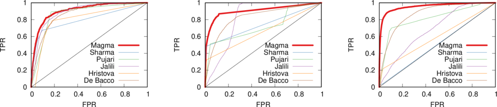
This is the real queen question of the post, and we do not fully answer it, unfortunately. However, we have a very good reason to think that the answer could be positive. We created a predictor which trains on 17 matches and then, given the global multi-layer network, will pick the winner. You can see the problem of the approach here: we use the network of the match as it happened to “predict” the outcome. However, we did that only because we did not have enough matches for each individual team: we believe we can first predict how pass and disruption networks will shape in a new match using historic data and then use that to predict the outcome. That will be future works, maybe if some team is intrigued by networks and wants to contact us for a collaboration… (wink wink).

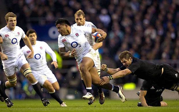
The reason I still like to report on our predictor is that it has a very promising property. Its accuracy was 83%. We compared with a prediction made with official rugby rankings, whose performance is worse: 76% accuracy. We also tested against bookmakers, who are better than us with their 86% accuracy. However, historic data on bets only cover more important matches — only 14 out of 18 — and matches between minor teams are usually less predictable. The fact that we are on par on a more difficult task is remarkable. More importantly, bookies tend to just “choose the best team”. For instance, they always predict a New Zealand win. The Haka, however, is not always enough and our networks caught that. New Zealand lost to England in a big upset on December 1st 2012. The bookmakers didn’t see that coming, but our network approach could have.

Continue Reading

As a kid from the 80s*, I remember how revolutionary the cellphone era was. It happened so fast. It seemed that, overnight, you could carry in your pocket a device connecting you to everybody you knew, no matter how far. To me, it changed everything. But did it? Yes, over-apprehensive parents can check their babies at the swipe of a finger, and whoever does not carry their cellphone with themselves at all times is labeled as a weirdo — I’m guilty of that. But the telecommunication revolution promised something more: the elimination of distance in communication. Did it deliver? This question was the motivation engine for the paper “Evidence That Calls-Based and Mobility Networks Are Isomorphic” which I wrote with my boss Ricardo Hausmann and which recently appeared in PLoS One.

The question is rather daring, so we decided to take it step by step. The simplest thing we came up was: let’s draw a map of cellphone calls and see if it looks like a geographical map. If it does, we might be onto something. To do so, we obtained data from telecommunication operators in Colombia. They provided us call detail records, where identifiers were encrypted to preserve the anonymity of the people making and receiving the calls. We also aggregated the data to make even the slightest re-identification impossible: every ID was associated to the municipality in which it spent most of its time and so all data was lumped together at the municipality level. At this point, we could draw a map of which municipalities had a significant call traffic with one another. This we called the “Call-based” network:

Click to enlarge

Before jumping to conclusions with this picture, we built a sister network. Since we just said we knew the location of a phone when making a call, we can keep a record of the different municipalities where we spotted the phone. Again, we joined together all data at the municipality level. This sister network is then a “Mobility” network of Colombia:

Click to enlarge

It seems there’s something here. The two networks appear to be similar: Bogotá seems to be a prominent center and the connections have a geographical component embedded into them. To make this more evident, we drew the networks on a Colombian map. The color of the municipalities is the same color of the nodes in the pictures above: nodes with the same color are very related in the network — network clusters.

Click to enlarge

The call-based network is on the left, the mobility is on the right. Blocks of the same color on the left are a clear indication of the call connections being influenced by geography. If there was no relation, the map would look like the Harlequin shirt, with colors scattered evenly across the territory. Mobility clusters are also short-range, although the pattern is harder to see because I had to use many more colors: the clusters are smaller. But the two networks are closely related: in fact, the larger call-based clusters contain the smaller mobility ones, as we show in the paper. We can say that there is a strong relationship between calls and mobility.

This is nice, because it fits with many works in computer science that actually use social relationships to predict human mobility… and vice versa. On the other hand, it is not nice because the existence of these papers also tells us ours is not a new result. Moreover, my starting point was to hint that the call-based and mobility networks are obeying the same laws, not that they are merely correlated. We need to go a step further.

Our step was to consider the difference that distance makes in the two networks. When looking at mobility, the distance between an origin and a destination is an important cost. In the call-based networks, things are a bit trickier. If modern telecommunication really delivered what it promised, distance should be a really low cost, and probably non-linear. To start a social relationship it is not needed to be in the same place at any given time, and even if we move to opposite ends of the world, we can still call each other. As a consequence, there shouldn’t be a way to scale the cost of distance in the call-based network to look like the one in the mobility network.

When we attempted to perform such scaling, we discovered it was actually possible. We checked, at any given distance, the ratio between commuters and callers. If two municipalities are at 50km distance, and there are twice as many commuters than callers, we have a dot on coordinates (50, 2). If we take two municipalities at 100km distance, and the commuters are just a third of the number of callers, the data point is at coordinates (100, .33). Once we consider all data points, we can fit our green line, AKA the scaling function from calls to mobility:

When we used this adjustment to calculate new call-based clusters using the distance cost “as if” it was the mobility network, we obtained the mobility clusters. We detail in the paper the reasons why this is not as circular as it seems.  In practice, our green line is a transformation function that morphs the call-based network into the mobility network. If modern telecommunication really killed distance, that green line shouldn’t exist, or at least it should be so wobbly to be practically useless.

There are many ways in which you could interpret this result. One that Ricardo and I like focuses on the relationship between face-to-face and electronic mediated meetings. It’s not like the people you call are the ones you really would rather meet but you cannot. It’s more like you call AND you meet, whenever it is possible. Face-to-face and electronic mediated meetings are not really substitutes in this world, they are more like complements. To come back to my opening, I’d say new technologies didn’t eliminate distance from the communication equation. Alleviate, yes. But ultimately, it’s more like an increased bandwidth than a revolution. At least so far.

* Shut up, I’m still in my twenties. Everybody knows 1996 was only 10 years ago.

Continue Reading

You need to forgive me for the infamous click-bait title I gave to the post. You literally need to, because you have to save your hate for the actual topic of the post, which is Big Data. Or whatever you want to call the scenario in which scientists are flooded with so much data that traditional approaches break, for one reason or another. I like to use the Big Data label just because it saves time. One of the advantages of Big Data is that it’s useful. Once you can manage it, simple analysis will yield great profits. Take Google Translate: it does not need very sophisticated language models because millions of native speakers will contribute better translations, and simple Bayesian updates make it works nicely.

Of course there are pros and cons. I am personally very serious about the pros. I like Big Data. Exactly because of that love, honesty pushes me to find the limits and scrutinize the cons of Big Data. And that’s today’s topic: “yet another person telling you why Big Data is not such a great thing (even if it is, sometimes)” (another very good candidate for a click-bait title). The occasion for such a shameful post is the recent journal version of my work on human mobility borders (click for the blog post where I presented it). In that work we analysed the impact of geographic resolution on mobility data to locate the real borders of human mobility. In this updated version, we also throw temporal resolution in the mix. The new paper is “Spatial and Temporal Evaluation of Network-Based Analysis of Human Mobility“. So what does the prediction of human mobility have to do with my blabbering about Big Data?

Big Data is founded on the idea that more data will increase the quality of results. After all, why would you gather so much data at the point of not knowing how to manage them if it was not for the potential returns? However, sometimes adding data will actually decrease the research quality. Take again the Google Translate example: a non native speaker could add noise, providing incorrect translations. In this case the example does not really hold, because it’s likely that the vast majority of contributions comes from people who are native speakers in one of the two languages involved. But in my research question about human mobility it still holds. Remember what was the technique in the paper: we have geographical areas and we consider them nodes in a network. We connect nodes if people travel from an area to another.

Let’s start from a trivial observation. Weekends are different from weekdays. There’s sun, there’s leisure time, there are all those activities you dream about when you are stuck behind your desk Monday to Friday. We expect to find large differences in the networks of weekdays and in the networks of weekends. Above you see three examples (click for larger resolution). The number of nodes and edges tells us how many areas are active and connected: there are much fewer of them during weekends. The number of connected components tells us how many “islands” there are, areas that have no flow of people between them. During weekends, there are twice as much. The average path length tells us how many connected areas you have to hop through on average to get from any area to any other area in the network: higher during weekdays. So far, no surprises.

If you recall, our objective was to define the real borders of the macro areas. In practice, this is done by grouping together highly connected nodes and say that they form a macro area. This grouping has the practical scope of helping us predict within which border an area will be classified: it’s likely that it won’t change much from a day to another. The theory is that during weekends, for all the reasons listed before (sun’n’stuff), there will be many more trips outside of a person’s normal routine. By definition, these trips are harder to predict, therefore we expect to see lower prediction scores when using weekend data.

The first part of our theory is proven right: there are indeed much less routine trips during weekends. Above we show the % of routine trips over all trips per day. The consequences for border prediction hold true too. If you use the whole week data for predicting the borders of the next week you get poorer prediction scores. Poorer than using weekday data for predicting weekday borders. Weekend borders are in fact much more volatile, as you see below (the closer the dots to the upper right corner, the better the prediction, click for higher resolution):

In fact we see that the borders are much crazier during weekends and this has a heavy influence on the whole week borders (see maps below, click for enjoying its andywarholesque larger resolution). Weekends have a larger effect on our data (2/7), much more than our example in Google Translate.

The conclusion is therefore a word of caution about Big Data. More is not necessarily better: you still need theoretical grounds when you add data, to be sure that you are not introducing noise. Piling on more data, in my human mobility study, actually hides results: the high predictability of weekday movements. It also hides the potential interest of more focused studies about the mobility during different types of weekends or festivities. For example, our data involves the month of May, and May 1st is a special holiday in Italy. To re-ignite my Google Translate example: correct translations in some linguistic scenarios are incorrect otherwise. Think about slang. A naive Big Data algorithm could be caught in between a slang war, with each faction claiming a different correct translation. A smarter, theory-driven, algorithm will realize that there are slangs, so it will reduce its data intake to solve the two tasks separately. Much better, isn’t it?

Continue Reading

The literature about community discovery, which deals with the problem of finding related groups of nodes in a network, is vast, interesting and full of potential practical applications. However, if I would have to give one critique of it, it would be about its self referential character. Most community discovery papers I read in computer science and physics journals are mainly about finding communities. Not much time is spent thinking about what to do with them, or what they mean. My first post in this blog was about a community discovery algorithm. Recently, an extended version of that paper has been accepted in a computer science journal. Since that first post, I (mainly) added some crucial modifications and features to the algorithm. I don’t want to talk about those here: they are boring. I also didn’t bring up this paper to boast about it. Okay, maybe a little. I did it because the paper touches upon the issue I am talking about here: it tries to do something with communities, it tries to explain something about them. Namely, it asks: why do communities overlap?

First of all: communities do overlap. When trying to detect them, many researchers realized that hard partitions, where each node can belong to one and only one community, are not always a good idea. Most of them found this a problem. Others were actually very happy: the problem gets harder! Nice! (Researchers are weird). Blinded by their enthusiasm, they started developing algorithms to deal with this overlap. Not many asked the question I am trying to answer here: why do communities overlap? As a result, some of these algorithms detect this overlap, but using approaches that do not really mean anything in real life, it’s just a mathematical trick. Others, instead, build the algorithm around a core hypothesis.

This hypothesis is nothing unheard of. Communities overlap because people have complex lives. Some of your college mates also attend your yoga class. And you know your significant other’s colleagues, which puts you in their community. All these communities have you as common member, and probably some more people too. The beauty of this is that it is not only intuitive: it works well in finding communities in real world social networks. So well that it is the assumption of my approach and of many others outstanding algorithms (this and this are the first two that pop into my mind, but there are probably many more). Another beautiful thing about it is that it is almost obvious, and so it is probably true. But here we hit a wall.

The fact that it is simple, reasonable and it works well in practice proves nothing about its property of being true. There are things that are not simple nor reasonable, but nevertheless true (hello quantum physics!). And there is practical knowledge that does not quite correspond to how things work (in my opinion, most computer science is a patch and nobody really knows why it works). Unless we test it, we cannot say that this nice practical principle actually corresponds to something happening in reality. So how do we go on and prove it? In the paper I proposed a first step.

This brings me back to another old love of mine. Multidimensional networks. They are networks in which we put multiple relations in a cage together in mating season and see what happens (research is fun). The idea behind the paper is that multidimensional networks give us the perfect tool to test the hypothesis. In monodimensional networks you have no clue why two people are connecting besides the obvious “they know each other”. In a multidimensional network, you know why they know each other, it’s information embedded in the type of the relation. So, the hypothesis is that different types of relations are the cause of the community overlap, and with multidimensional networks we can look at how communities distribute over relations. First, let us take a look at what two overlapping communities look like in a multidimensional network.

We collected a multidimensional social network putting together relationships between users in Facebook, Twitter and Foursquare. We then used DEMON to extract overlapping communities from each dimension. We then took two communities with extensive overlap in the Facebook dimension (picture below).

We then looked at the very same set of nodes, but now in the Foursquare network. In the picture below, we kept the edges, and the node positioning, of the Facebook network to make the comparison easier, but keep in mind that the edges in the Foursquare dimension are different, and they are the ones that decide to what community the nodes belong.

Very interesting. The communities look a lot alike, although the shared (and non shared) nodes are slightly different. Now node 7369 is shared (it wasn’t in Facebook) while node 8062 isn’t (whereas it was before). Let’s put another nail on the coffin and see the communities these nodes belong in Twitter (same disclaimer applies):

Surprise surprise, in Twitter there is actually only one community, which brings together the majority of the nodes of the two communities. So here’s where our overlap comes from: common affiliations in different dimensions! Now, I’m going to deal with that voice in your head that is screaming “Anecdotal! Anecdotal!”. (You don’t hear it? Did I already mention that researchers are weird? In any case “Anecdotal” refers to a type of evidence that bears no value in scientifically proving a point if not backed by more solid proofs). Put in a more general way: the more two communities overlap in some dimension, the more likely it is we can find a dimension in which these communities are actually a single community. This involves boring details you can find in the paper which ultimately generate this plot:

Does this plot prove our theory without leaving out any reasonable doubt? Maybe, or not really. There are still things to check. But science is made by tiny steps forward. And this is certainly one.

Continue Reading

Today I want to talk about jobs. Or, better, about finding a job. Sooner or later, this is a task that many people will have to perform and it is not usually a very enjoyable one. Writing a CV is mostly painful. You have to list all your skills, all the knowledge you have, what you have done in the past, the tasks you can perform. Everything to maximize your value to the eyes of the examiner, who is judge, jury and executioner of your working fate. But, after all, you can’t complain. You know the rules of the game. It is only fair, because the recruiter wants to see the best possible CV and the best possible CV is the one that includes the most relevant information: you have to stuff the maximum amount of skills in your body to maximize your value and it is the most valuable person the one who is going to be picked. Right?

Wrong. There’s one critical flaw to that reasoning, and that is time. Time is limited. You can’t spend too much time in stuffing knowledge into you, because there is too much knowledge out there and if you try to internalize everything you don’t have time to produce anything. This is not just my opinion. It is one of the cornerstones of widely accepted and useful theories, for example the division of labour. This is linked to the concept of “social knowledge“. Social knowledge is the collection of what people in society know. While personal knowledge is bounded by time, social knowledge is not, because many different brains work on it at the same time, making it grow beyond what any individual can grasp.

If you want to have 100 people to make cars, you don’t teach each one of them to make a car from scratch and then you watch them making 100 cars at the same time. Each guy will assemble one part. And he’ll be awesome at that particular part. This applies not only to manufacturing. How many times in your working life you found yourself struck with a problem, not exactly in your knowledge domain, and you solved it by simply asking someone about it? In my case, many. Think about how many times you Google something. That’s accessing the social knowledge of humanity. That is one of the reasons why, for example, the social return of education exceeds the private return.

The way you access social knowledge also changes the usefulness of it. It is better if a friend takes time to explain things to you than if you have to read an answer in Quora, that is also related only to some extent to your specific problem. Because tacit knowledge needs a broker to make it explicit and understandable. So it is better to have knowledgeable friends in many fields, or: your social network matters for your qualifications, because it’s the principal medium you use to get explicit knowledge from the tacit social knowledge.

So it seems like we are onto an interesting problem. On one hand, I hope to have convinced you that social knowledge is an important component of someone’s value; on the other hand that creates more questions than answers. How do we evaluate a person for a job? How do we measure the social knowledge she has access to? Well, if you know me you know what’s going to happen. A network algorithm, of course! Precisely, an algorithm with a flavor of Philip K. Dick in its name: UBIK, or “U know Because I Know”. This algorithm has been created and developed with the help of Giulio Rossetti, Diego Pennacchioli and Damiano Ceccarelli and has resulted in a paper published in the ASONAM 2013 conference that will take place later this month. Also, the code of UBIK is available for use.

Here’s how UBIK works. First, you have to start by collecting information about the social connections of people. It’s even better if you can find multiple types of connections from multiple sources, because the channel through which knowledge passes influences the quality of that knowledge. Second, for each person you have to collect their CV. Personal knowledge is still important. Once you have these pieces of information, UBIK can unweave its magic.

Let’s look at a simple example. The above picture can be considered a network of people: each node is a person, each person is connected to the people she knows, her color represents the skill in which she is specialized, and the width of the link is the strength of the connection (important: UBIK works with qualities of links, not strengths, but for the sake of simplicity in this example we use the latter). The consequence of our theory is that the skills of each person are transferred through the links of the network. Also, a direct connection is stronger than a connection through another node. For example, node 8 passes her skills more efficiently to 1 than node 10 does.

So, at the first iteration, UBIK passes the skills of each node to its neighbors. Node 1 gets a lot of red skill, node 10 gets all kinds of skills. It is a percolation process. At each iteration, UBIK keeps passing the entire set of updated skills, with an increasing penalty due to the social distance. I won’t bother you with the equations. Just know that, at some point, the penalty is so high that the algorithm stops.  The skill transfer happens proportionally to the strength of the links connecting the nodes. As a result, node 10 is super valuable, because she has access to the knowledge about all skills in the network, while for example node 1 will be a uber-specialist of the red skill. By just looking at their CV, it would be impossible to extract this information.

Some of you familiar with network analysis may have some bells ringing in their heads. “This is node ranking!” Well, yes. “So just use PageRank!” “Or HITS!” “Why do we need UBIK?” Well, for a number of reasons. First, UBIK handles multiple link types and multiple skills at the same time: (variants of) PageRank and HITS can do one or the other, but not so many can do it simultaneously yielding effective results. Second, PageRank and HITS have flaws. PageRank correlates with degree (the number of connections of a node) and centrality measures: see the above picture where we confront the rankings of the algorithms with the degree rank. HITS has similar flaws related to the nodes’ tendency of cluster in communities.

Moreover, when we applied the algorithms to network of researchers, UBIK was most likely to rank them in the same way as measures independent from networks such as the H-Index. This shows that UBIK may be more useful than other network ranking techniques when these independent evaluation criteria are not available. The beauty of UBIK consists in multiple rankings. Below I report some rankings of researchers in Computer Science. Each number is the rank that UBIK gave to the researcher in a particular conference. Each conference is a different ranking that UBIK is able to distinguish. We are able to spot the specialists of many computer science conferences, highlighting their prominence in one community and low ranking in others. Also, we report the rankings in these conferences for the most prominent general authors, showing that they rank on average well in many different venues, but they are not really specialists.

And that’s why you should give UBIK a chance.

Continue Reading

The real world has many important characteristics. One I heard being quite salient is the fact that time passes. Any picture of the world has to evolve to reflect change, otherwise it is doomed to be representative only of a narrow moment in time. This is quite a problem in computer science, because when we want to analyze something we need to spend a lot of time in gathering data and, usually, the analysis can be done only once we have everything we need. It’s a bit like in physics, when the problems are solved in the vacuum and in the absence of friction. Of course, many people work to develop dynamics models, trying to handle the changes in the data.

Take link prediction, for example. Link prediction is the branch of network science whose aim is to predict which connections are more likely to appear in the near future, given the current status of a network. There are many approaches to this problem: one simply states that the probability that two nodes will connect is proportional to their current degree (because it’s being observed that high degree nodes attracts more edges, it’s called “preferential attachment“), another looks at the history of the new edges which came into existence and tries to redact some evolution rules (see the paper, not much different from my work on signed networks).

What’s the problem in this? The problem lies in the fact that any link came into existence in a specific moment, in which the network shape was different from any other moment. Let’s consider the preferential attachment, with an example. The preferential attachment tells you that the position in the market of Google not only is not in danger: it will become stronger and stronger, because its high visibility attracts everybody who needs the services it is providing. However, Google was not born with the web, but several years after. So in the moment in which Google was born, the preferential attachment would have told you that Google had no chance to beat Yahoo. And now it’s easy to laugh at this idea.

So, what happened? The idea that I investigated with my colleagues at the KDDLab in Italy is extremely simple: just like Earth’s geological times, also complex networks (and complex systems in general) evolve discontinuously, with eras in which some evolution rules apply and some others, valid in other eras, don’t. The original paper is quite old (from 2010), but we recently published an update journal version of it (see the Intelligent Data Analysis Journal), that’s why I’m writing about it.

In our paper, we describe how to build a framework to understand what are the eras in the evolution of a network. Basically, everything boils down to have many snapshots of the network in different moments of time and a similarity measure that tells you how similar are two consecutive snapshots. Then, by checking the values of this similarity function, one can understand if the last trends she is seeing are providing reliable information to make predictions or not. In our world, then, we understand that when Google enters in the web anything can happen, because we are in a new era and we do not use outdated information that do not apply anymore to the new scenario. In our world, also, we are aware that nobody is doomed to success, regardless how good its current position is. A nice and humbling perspective, if I may say.

I suggest reading the paper to understand how nicely our era detection system fits with the data. The geekier readers will find a nice history of programming languages (we applied the era discovery system to the network of co-authorship in computer science), normal people will probably find more amusement in our history of movies (from networks of collaboration extracted from the Internet Movie Database).

So, next time you’ll see somebody trying to make predictions using complex network analysis, check if she is considering data history using an equivalent of our framework. If she does, thumbs up. If she doesn’t, trust her just like you would trust a meteorologist trying to forecast tomorrow’s weather by crunching data from yesterday down to the Mesozoic.

Continue Reading

I decided to give to this blog post an obscure title because today I want to talk about something that in complex network analysis goes under many names, so I did not want to favor any of them. What I am talking about are networks with multiple types of relations in them, the main subject of my PhD Thesis and of a recent article that I published in the World Wide Web Journal. These structures are putting more complexity on top of complex networks, therefore they are complex network squared: hence the fancy blog title.

These networks are referred to in the literature with the following terms:

• Multidimensional (the term that I use in my thesis);
• Multirelational;
• Layered;
• Interdependent;
• Multisliced;
• Multilevel;

and so on and so forth. All these terms refer to the same theoretical object, that is also implemented in many ways. I’ll mention some of them just to sound like the guardian of an obscure cult: labeled multigraphs, hypergraphs, mesostructures and coupling edges.

Despite the confusion that I tried to create with the first paragraphs, the general idea of this line of research is brutally simple: in our everyday life we are not part of only one network. It may look like we are, but when we start thinking harder about our relationships, we realize that we know the people we know for different reasons. This idea is the one behind the fact that every person can belong to different “communities” at the same time, which I already discussed in these pages. But it is deeper than that. It does not only require the more sophisticated, but still traditional, community discovery algorithm that I described in that blog post. It requires a whole new model and mindset.

Before multidimensional networks (forgive me if for clarity I’ll use my term for these structures) the classical complex network analyst would just assume that a single relation represents a particular phenomenon and nothing else can be said about it. Allow me to recycle this picture about my Facebook friends:

Intuitively this looks nice, as we can find communities and central nodes. But is this picture really telling us everything about my Facebook friends? What about a higher order of aggregation among them? What about not only their friendship links but also their common interests? The multidimensional network analyst throws a bunch of new connections on top of it and she tells you: “There’s something more”. In this case:

A visualization that is not nearly as elegant as the previous one, I give you that, but nevertheless it is useful to understand a higher level aggregation of my Facebook friends. On top of the connections between friends, we added edges connecting people if they are part of the same group or if they like the same stuff on Facebook. The two gigantic hairballs are composed by people who are in the same location: there is the cluster of people living in Italy, the one of people living in the US, and connections between them from people travelling between the two countries. So, we saw that adding different types of relations uncovers structural properties that none of the relations by itself would reveal.

I’ll give you another example of a cool real world effect of multidimensional networks. This is not from a work of mine, but it is from the Nature paper “Catastrophic cascade of failures in interdependent networks” by  Sergey V. Buldyrev, Roni Parshani, Gerald Paul, H. Eugene Stanley and Shlomo Havlin. Suppose you have a power grid: what happens if one plant is subject to a failure? The classical complex network analyst tells you that we could not care less: the power grid is a scale free network, in which the majority of plants are only connected to a couple other plants. So, a random failure of one plant does not affect the rest of the network too much, unless we are extremely unlucky and we lose a power hub (but that’s really rare, and the classical network guy is an incurable optimist).

A multidimensional network scientist, instead, is way more careful. Why? Because he knows that the power grid network is not independent from everything else, but it is plugged into another network. For example, in a computer network that regulates its functioning. When a power plant goes down, a set of computers cannot work anymore. And what happen to the plants that are connected to those computers? They fail too, triggering another computer failure and God helps us all. It is theoretically proven that two different scale free relations, dependent on each other, are much much much more fragile than a single scale free network. This actually happened in Italy (where else?) and the following is a depiction from Buldyrev et al’s paper:

In the first Italy we see one plant going down (in red on the map) taking with it the computers it supplies with energy (in the flying network). This triggers a couple more failures in the second picture that eventually, in the third picture, completely destroy the power supply chain of southern Italy.

So far I gave you the idea that multidimensional networks are not exactly the same animal as classical complex networks. To give you a taste of how to prove this, I’ll spare you the super complicated equations of interdependent network percolation present in the Nature paper. I’ll instead provide another example from community discovery. As I said in my previous post, community discovery is loosely defined as the problem of grouping nodes in a network that are “densely connected”. Naturally, when we deal with multidimensional networks, the “densely connected” has to be changed into “multidimensionally densely connected”. Why is this challenging? Here I’ll give you an intuition and I promise that in the future I’ll come back with more details. For now, it is sufficient to use two pictures. Here’s the first:

Here we assume that we have two different dimensions and they are represented with solid or dashed edges. Is this set of nodes multidimensionally dense? Of course: everybody is connected with everybody and all dimensions of the network are equally represented. Now consider another situation:

Is this set of nodes multidimensionally dense? Of course: everybody is connected with everybody and all dimensions of the network are equally represented. But the two examples are very different. That’s funny: we just discovered that, in multidimensional networks, density is an ambiguous concept.

And, as conclusion, I’ll add some multidimensional flavor to another classical network problem: link prediction. Link prediction aims at predicting your next Facebook friend. The above mentioned multidimensional network scientist steps in and says: “But why only your next Facebook friend? Why not your next virtual acquaintance tout-court?”. He means that all your social media connections and their different types play a role in determining when and where you’ll connect with somebody. This is exactly what multidimensional link prediction is, and how to do this is a complex problem that currently remains unsolved. But the multidimensional network guy loves complex problems as much as he loves complex words.

Continue Reading